| Date | Notes |
| Tuesday 08/24 | Introductions, course policies. Syllabus.
Inspirational reading: AI@UF;
UF AI Initiative;
UF first US university to acquire world's most advanced AI system.
Motivational reading: Physics Careers: the Myths, the Data and Tips for Success; invited talk at the Career Forum of the Pheno 2020 conference.
|
| Tuesday 08/24 |
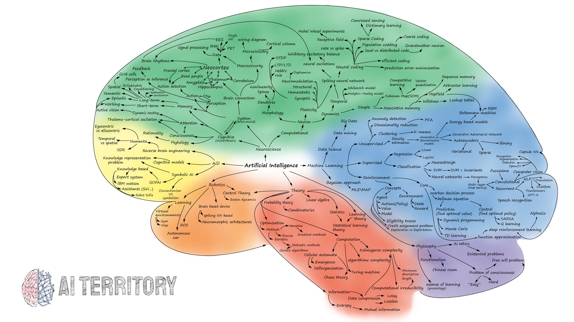
What is data science? Brief outline of the main topics to be covered in the course.
A map of AI topics from a
blog by a former physicist.
Discussion of final projects.
Introduction to Google Colab. Getting set up.
|
| Thursday 08/26 |
PYTHON TUTORIAL Python tutorial 00. Introduction 01. How to run python code 02. A quick tour of python language syntax 03. Basic python semantics: variables and objects 04. Basic python semantics: operators 05. Built-in scalar types: simple values 06. Built-in data structures 07. Control flow. 08. Defining and using functions 09. Errors and exceptions. 10. Iterators 11. List comprehension 12. Generators 13. Modules and packages 14. String manipulation and regular expressions 15. A preview of data science tools 16. Resources for further reading
Action items: by our next class (Thuesday), try going over all 16 sections. More python exercises and quizzes (with answers) are available here. |
| Tuesday 08/31 |
NUMPY TUTORIAL NumPy tutorial. Begin reading Chapter 2 "Introduction to NumPy". 2.1. "Understanding Data Types in Python" A Python List Is More Than Just a List, Fixed Type Arrays in Python, Creating Arrays from Python Lists, Creating Arrays from Scratch. 2.2. "The Basics of NumPy Arrays" NumPy Array Attributes, Array Indexing: Accessing Single Elements, Array Slicing: Accessing Subarrays, Subarrays as no-copy views, Creating copies of arrays, Reshaping of Arrays, Array Concatenation and Splitting. 2.3. "Computation on NumPy Arrays: Universal Functions" The Slowness of Loops, Introducing UFuncs, Exploring Numpy's UFuncs: array arithmetic, absolute value, trigonometric functions, exponents and logarithms, specialized ufuncs. 2.4. "Aggregations: Min, Max, and Everything In Between" Summing the Values in an Array, Minimum and Maximum, Multidimensional aggregates, Example: What Is the Average Height of US Presidents? |
| Tuesday 08/31 |
NUMPY TUTORIAL 2.5. "Computation on Arrays: Broadcasting" Introducing broadcasting. Fig. 2-4 Visualization of NumPy broadcasting. Rules of broadcasting. (skip the rest of that section) 2.6. "Comparisons, Masks, and Boolean Logic" Skip "Example: Counting Rainy Days in Seattle". Go over: Comparison operators as ufuncs. Working with Boolean arrays. Skip the rest. 2.7. "Fancy Indexing" (skip this section) 2.8. "Sorting Arrays" Read: Fast Sorting in NumPy: np.sort and np.argsort. Sorting along rows or columns. Skip ther rest: Partial sorts: Partitioning. Example: k-Nearest neighbors. 2.9. "Structured Data: NumPy's Structured Arrays" (skip this section) Programming practice: NumPy exercises. |
| Thursday 09/02 |
PLOTTING TUTORIAL Matplotlib tutorial: 04-01. Simple Line Plots. Adjusting the Plot: Line Colors and Styles. Adjusting the Plot: Axes Limits. Labeling Plots. Aside: Matplotlib Gotchas. 04-02. Simple Scatter Plots. Scatter Plots with plt.plot. Scatter Plots with plt.scatter. plot Versus scatter: A Note on Efficiency. 04-03. Visualizing Errors. Basic Errorbars. [Skip: Continuous Errors] 04-04. Density and Contour Plots. Visualizing a Three-Dimensional Function. 04-05. Histograms, Binnings, and Density [to fix the error, replace normed=True with density=True] Two-Dimensional Histograms and Binnings. [Skip: Kernel density estimation] 04-06. Customizing Plot Legends. [the rest of this section is optional] Choosing Elements for the Legend. Legend for Size of Points. Bug fix: use the full URL address of the data file with California cities data: https://raw.githubusercontent.com/jakevdp/PythonDataScienceHandbook/master/notebooks/data/california_cities.csv Skip: Multiple Legends. 04-07. Customizing Colorbars. [the rest is optional] Color limits and extensions. Discrete Color Bars. Example: Handwritten Digits. 04-08. Multiple Subplots. plt.axes: Subplots by Hand. plt.subplot: Simple Grids of Subplots. [the rest is optional] plt.subplots: The Whole Grid in One Go. plt.GridSpec: More Complicated Arrangements. 04-09. [optional] Text and Annotation. Example: Effect of Holidays on US Births [Use the full address for the data file https://raw.githubusercontent.com/jakevdp/data-CDCbirths/master/births.csv]. Transforms and Text Position. Arrows and Annotation. 04-10. [optional] Customizing Ticks. Hiding Ticks or Labels. Major and Minor Ticks. Reducing or Increasing the Number of Ticks. Fancy Tick Formats. 04-11. Customizing Matplotlib: Configurations and Stylesheets. [Skip: Plot Customization by Hand [if you decide to try it, replace ax = plt.axes(axisbg='#E6E6E6') with ax = plt.axes(facecolor='#E6E6E6') to fix the error]. Changing the Defaults: rcParams. Stylesheets. 04-12. [optional] Three-Dimensional Plotting in Matplotlib. Three-dimensional Points and Lines. Three-dimensional Contour Plots. Wireframes and Surface Plots. Surface Triangulations. Example: Visualizing a M�bius strip. Skip the remaining sections 04-13 to 04-15. |
| Tuesday 09/07 |
5.02. Introducing Scikit-Learn. Data Representation in Scikit-Learn: features and samples, features matrix, target array. Scikit-Learn's Estimator API.
Programming practice: Loading and plotting the standard datasets. Playing with the parameters. Matplotlib exercises. |
| Tuesday 09/07 |
STATS WEEK Statistics 101: Exploratory data analysis. Key terms for data types: continuous, discrete, categorical, binary, ordinal. Key terms for rectangular data: data frame, feature, outcome, records. Non-rectangular data structures. Key terms for estimates of location: mean, weighted mean, median, weighted median, trimmed mean, outliers, robustness. Key terms for variability metrics: deviations, variance, standard deviation, mean absolute deviation, median absolute deviation from the median, range, order statistics, percentile, interquartile range (IQR). Key terms for distribution shapes: boxplot, frequency table, histogram, density plot, violin plot, contour plot. Key terms for categorical data: mode, expected value, bar charts, pie charts. Key terms for correlation: correlation coefficient, correlation matrix, scatterplot. |
| Thursday 09/09 |
Statistics 102: 2. Data and sampling distributions. 2.1. Random sampling and sample bias. Population. Sample. Random and stratified sampling. Bias. Random selection. Sampling with replacement. Sampling without replacement. Sample mean versus population mean. Sample size versus sample quality. 2.2. Selection bias. Vast search effect. Data snooping. Regression to the mean. |
| Tuesday 09/14 |
Statistics 102: 2.3. Sampling distribution of a statistic. Sample statistic. Data distribution. Sampling distribution. Central limit theorem. Standard error. 2.4. The bootstrap. Bootstrap sample. Resampling. Jackknife. 2.5. Confidence intervals. Confidence levels. Interval endpoints. 2.6. Normal distribution. z-score. Standard normal. QQ-plot. 2.7. Long-tailed distributions. 2.8. Student's t-distribution. 2.9. Binomial distribution. Trial. Success. Probability of success. 2.10. Poisson and related distributions. Exponential distribution. |
| Tuesday 09/14 |
Statistics 103: 3. Statistical experiments and significance testing. 3.1. A/B testing. Treatment, treatment group, control group, randomization, subjects, test statistic, blind study, double blind study. 3.2. Hypothesis tests. Null hypothesis, alternative hypothesis, one-way and two-way hypothesis tests. 3.3. Resampling. The bootstrap. Permutation test. 3.4. Statistical significance and p-values. P-value, Alpha, Type 1 and type 2 errors. 3.6. Multiple testing. Look-elsewhere effect. Adjustment of p-values. 3.9. Chi-square test. Pearson residuals. 3.10. Multi-arm bandit problem. Exploration&exploitation tradeoff dilemma. A few strategies: epsilon-first; epsilon-greedy, epsilon-decreasing. PANDAS: Chapter 4 of the book. (optional) |
| Thursday 09/16 |
Programming practice: Loading and plotting datasets. Manipulating numerical data.
Loading datasets. 1. Loading from scikit-learn. 2. Loading with seaborn. 3. Generating a dataset on the fly. 4. Loading an existing dataset from a csv file. 5. Rescaling a feature. 6. Standardizing a feature. 7. Generating polynomial and interaction features. Handling missing data. |
| Tuesday 09/21 |
05-01. What is Machine Learning? Examples of: Supervised learning: classification and regression. Unsupervised learning: clustering and dimensionality reduction. 5.02. Introducing Scikit-Learn: Data Representation in Scikit-Learn: features and samples, features matrix, target array. Scikit-Learn's Estimator API. |
| Tuesday 09/21 |
Continue 5.02. Introducing scikit-learn. Supervised learning example: Simple linear regression, fit() and predict() methods. Supervised learning example: Iris classification [bug fix: replace cross_validation with model_selection], accuracy score. Unsupervised learning example: Iris dimensionality. |
| Thursday 09/23 |
Continue 5.02. Introducing scikit-learn. Unsupervised learning: Iris clustering [bug fix: replace GMM with GaussianMixture]. Application: Exploring Hand-written Digits: - Dimensionality reduction [bug fix: replace spectral with Spectral or another valid color map]. - Classification on digits, confusion matrix. 5.03. Hyperparameters and model validation. How to train and validate with finite amount of data: simple examples. |
| Tuesday 09/28 |
Continue 5.03. Hyperparameters and model validation. Thinking about Model Validation: Holdout sets, Model validation via cross-validation [bug fixes: change cross_validation to model_selection and also change cv=LeaveOneOut(len(X)) to cv=LeaveOneOut() ]. Selecting the Best Model. The Bias-variance trade-off. Validation curve. Validation curves in Scikit-Learn [bug fix: replace "from sklearn.learning_curve import validation_curve" with "from sklearn.model_selection import validation_curve"]. Learning curves. Learning curves in Scikit-Learn. Validation in Practice: Grid Search [bug fix: replace "from sklearn.grid_search import GridSearchCV" with "from sklearn.model_selection import GridSearchCV"] [bug fix: delete the "hold=True" argument]. Weekend reading: 5.04. Feature Engineering. [bug fix: replace "from sklearn.preprocessing import Imputer" with "from sklearn.impute import SimpleImputer" and from then on use SimpleImputer instead of Imputer.] Categorical features: one-hot encoding, sparse matrices. Text features: word counts, term frequency-inverse document frequency. Derived features: basis function regression, polynomial features. Imputation of missing data. Feature pipelines: PolynomialFeatures+LinearRegression. |
| Tuesday 09/28 |
5.06. In Depth: Linear regression. Simple Linear Regression. Loss function for linear regression. Minimizing the loss function. Basis function regression. Polynomial basis functions. Gaussian basis functions. Regularization. Ridge regression (Tikhonov regularization), Lasso regularization, Elastic-net regularization. Skip: Example: Predicting Bicycle Traffic. Programming practice and homework: Linear Regression Challenge. |
| Thursday 09/30 |
5.05. In Depth: Naive Bayes Classification. Bayesian Classification: Bayes theorem, generative models. Gaussian Naive Bayes. Predicting the posterior probabilities. Multinomial Naive Bayes. Example: classifying text. When to Use Naive Bayes. Team exercise: classifying text for a different set of newsgroups.
Programming practice and homework: NB Classification Challenges. |
| Tuesday 10/05 |
5.07. In Depth: Support vector machines. Motivating Support Vector Machines: generative versus discriminative classification. Support Vector Machines: Maximizing the Margin: fitting a support vector machine, support vectors, kernel SVM, tuning the SVM: softening the margins. Homework example: Face Recognition. [bug fixes: use "from sklearn.decomposition import PCA as RandomizedPCA"; "from sklearn.model_selection import train_test_split"]
Programming practice and homework: SVM Challenges. |
| Tuesday 10/05 |
5.11. In Depth: k-means clustering. Introducing k-Means. k-means Algorithm: Expectation-Maximization. Caveats: sensitivity to the initial guess, number of clusters a priori unknown, works best with linear boundaries. SpectralClustering. Homework examples: k-means on digits; k-means for color compression. Further reading: Selecting the number of clusters with silhouette analysis on KMeans clustering. Background reading: |
| Thursday 10/07 |
5.12. In Depth: Gaussian-Mixture Models. Motivating GMM: Weaknesses of k-Means.
Generalizing E-M: Gaussian Mixture Models. Choosing the covariance type. GMM as density estimation.
How many components? Akaike and Bayesian information criteria.
Bug fixes: replace from sklearn.mixture import GMM gmm = GMM(n_components=4).fit(X) with from sklearn import mixture gmm = mixture.GaussianMixture(n_components=4).fit(X) Also replace for pos, covar, w in zip(gmm.means_, gmm.covars_, gmm.weights_): with for pos, covar, w in zip(gmm.means_, gmm.covariances_, gmm.weights_): Also replace Xnew = gmm16.sample(400, random_state=42) with Xnew, Ynew = gmm16.sample(400) Programming practice and homework: Clustering Challenges. |
| Tuesday 10/12 |
5.08. In Depth: Decision trees and random forests. Ensemble methods. Motivating Random Forests: Decision Trees. Creating a decision tree. Decision trees and overfitting. Ensemble of Estimators: Random Forests. BaggingClassifier. Random Forest Regression. Homework example: Random Forest for Classifying Digits. Programming practice and homework: Decision Trees and Random Forests Challenges. |
| Tuesday 10/12 |
The need for dimensionality reduction. The curse of dimensionality. Scaling of points in hypercubes of diferent dimensions. Main approaches for dimensionality reduction: projection and manifold learning.
5.09. In Depth: Principal Component Analysis. Introducing Principal Component Analysis. Components and explained variance. PCA as dimensionality reduction. PCA for visualization: Hand-written digits. [Bug fix: 'spectral' -> 'Spectral'] What do the components mean? Choosing the number of components. PCA as noise filtering. Example: Eigenfaces. Bug fix: replace from sklearn.decomposition import RandomizedPCA with from sklearn.decomposition import PCA as RandomizedPCA Programming practice and homework: PCA Challenges. |
| Thursday 10/14 |
Bonus Discussion on Dimensionality Reduction Using Feature Extraction. Linear Discriminant Analysis (LDA), Kernel PCA.
5.10. In Depth: Manifold Learning. Manifold Learning: "HELLO". Multidimensional Scaling (MDS). MDS as Manifold Learning. Nonlinear Embeddings: Where MDS Fails. Nonlinear Manifolds: Locally Linear Embedding. Example: Isomap on Faces. Example: Visualizing Structure in Digits. Bug fix: replace from sklearn.datasets import fetch_mldata mnist = fetch_mldata('MNIST original') with from sklearn.datasets import fetch_openml mnist = fetch_openml('mnist_784') mnist.target = mnist.target.astype(np.int8) # fetch_openml() returns targets as strings Programming practice and homework: Manifold Learning Challenges. |
| Tuesday 10/19 |
Density estimation as an unsupervised task. Density estimation from the Voronoi Tessellation.
5.13. In Depth: Kernel Density Estimation. Motivating KDE: Histograms. Kernel Density Estimation in Practice.
Selecting the bandwidth via cross-validation.
Bug fixes: replace |
| Tuesday 10/19 |
Bonus review of unsupervised learning techniques.
A few more clustering algorithms: Mean-shift, DBSCAN, agglomerative hierarchical clustering. Comparing different clustering algorithms on toy datasets. Further reading: Review of the material covered so far. A map of AI topics. The class resources.
Discussion of the choices for final projects. Scikit-learn examples database.
Machine Learning hackathons. The ML4SCI 2020 Hackathon. Publicly available datasets from your own (field of) research. Journal club?
Discussion of previous homework assignments.
Bonus topic: Comparison of supervised classifiers. Background reading: |
| Thursday 10/21 | Gradient Descent Methods (Chaper 4 in Geron). Selecting and training a model. Minimizing the loss function with respect to the hyperparameters. Analytical minimization of the loss function for linear regression. Normal equation. Numerical example, scikit-learn implementation. Gradient descent: the basic idea. Learning rate. Gradient descent pitfalls. The importance of scaling the features. Batch, stochastic and mini-batch gradient descent. Bonus: Why momentum really works. |
| Tuesday 10/26 |
Must-watch video: Neural Networks series at 3blue1brown. Legacy of neural network research in Physics at UF: R. Field. Deep learning: overview. Keras. Introduction to neural networks. Artificial neuron. Inputs, weights, connections, bias, activation function, output. The basic structure of a neural network: input layer, output layer, hidden layers. Backpropagation and gradient descent. |
| Tuesday 10/26 |
An example of a basic neural network: classifying the handwritten digits from the MNIST dataset. Variations in the network architecture: different choices for the activation function, the loss function, the optimizer, the metrics. Hyperparameters: learning rate, regularization, momentum. Available datasets in Keras. Must-watch video: Alphago: The Movie. |
| Thursday 10/28 |
No class lecture. Instead, attend the Physics Department colloquium on Machine Learning at 3 pm in NPB 1002:
Speaker: Sergei Gleyzer (University of Alabama) Abstract: The Large Hadron Collider (LHC) is delivering the highest energy proton-proton collisions ever recorded in the laboratory, permitting a detailed exploration of elementary particle physics at the highest energy frontier. It is uniquely positioned to detect and measure the rare phenomena that can shape our knowledge of new interactions and possibly resolve the present tensions of the Standard Model. LHC experiments have already observed the long-sought after Higgs boson and have achieved unprecedented levels of sensitivity to new particles at the TeV scale with on-going searches for new physics, including dark matter. This trend is expected to continue during the next LHC run and with the High-Luminosity Large Hadron Collider (HL-HLC), anticipated to start data taking in 2027. New ideas for event reconstruction and data analysis are required to address the experimental challenges posed by the complex experimental environment at the HL-LHC that arises from a significant increase in pile-up, or extra particle collisions of protons traveling in the same bunch, leading to far more complicated event signatures at the HL-LHC. In my talk, I will discuss the application of state-of-the-art machine learning methods to new physics searches at the LHC, detector reconstruction, event simulation and real-time event filtering at the LHC. I will also discuss related cross-over machine learning applications to searches for dark matter substructure with strong gravitational lensing with the upcoming Vera Rubin Observatory. |
| Tuesday 11/02 |
General guidelines for building neural networks. Different choices for the architecture and the hyperparameters. Example: Toy classification with Tensorflow. Example: Binary classification of the IMDB dataset. |
| Tuesday 11/02 | How to deal with overfitting: lower the network capacity, add weight regularization, add dropout. |
| Thursday 11/04 | Convolutional neural network (convnet). Example: classifying the MNIST digits. |
| Tuesday 11/09 |
Example: multiclass classification of Reuters newswires. Example: regression on the Boston housing price market. |
| Tuesday 11/09 |
ML4SCI hackathon. Slides from the kick-off meeting yesterday. The six challenges: 1. Identifying the Higgs boson 2. Classification of particle images (plus a bonus challenge) 3. Gravitational lensing (two tasks: classification and regression) 4. NMR spin challenge 5. Planetary albedo challenge 6. Circumgalactic medium challenge Bonus lecture: "Introduction to Machine Learning" Harrison Prosper (FSU) (2:30 pm), zoom link. |
| Thursday 11/11 |
No class: Veterans day. |
| Tuesday 11/16 |
Autoencoders. Latent representations (codings). Latent space. Undercomplete autoencoders. Example 1: simple autoencoder. Example 2: variational autoencoder. |
| Tuesday 11/16 |
Generative adversarial network (GAN). Basic architecture: the generator and the discriminator. Adversarial training. Training the discriminator. Training the generator. Examples: 1) PCA with an undercomplete linear encoder; 2) stacked autoencoder - training all at once or one at a time, tying weights, visualization, latent space vector arithmetic; 3) convolutional autoencoder; 4) recurrent autoencoder (skip); 5) denoising autoencoder; 6) sparse autoencoder (skip); 7) variational autoencoder. Examples: Simple GAN, deep convolutional GAN trained on the Fashion MNIST dataset. Results. |
| Thursday 11/18 |
EXAM |
| Tuesday 11/23 | Symbolic regression. |
| Tuesday 11/23 |
Review of Hipergator capabilities:
ML hackathon competitions: kaggle.
Final instructions for the final project presentations. Special high-energy seminar on AI: J. Thaler (MIT and IAIFI). You can watch the recording here. |
| Thursday 11/25 |
No class: Thanksgiving. |
| Tuesday 11/30 |
Rubric (30 pts total): 1. Introducing the topic [10]: what is the question we are trying to answer? Why is it important? Previous approaches - pros and cons. Why do we expect a (new) ML method would help in this case? 2. Machine learning aspect [10]: what ML technique was applied, what dictated the choice of this particular technique, rough description of the technique, choice of hyperparameters, training/validation (if applicable), results, conclusions. 3. Overall impression [5] and time management [5]: optimal mix of text/graphics/formulas, no spelling and grammar mistakes, appropriate font size, labelling the plots/axes, effective use of color/illustrations; finish within the alloted time of 12 min + 3 min for questions. The deadline for preparing the final projects is today. Everybody should be ready to present the final project TODAY, on November 30. The order of speakers will be chosen randomly before today's class. Final project presentations: session 1 (4 talks). Starts at 11:30 am. |
| Tuesday 11/30 | Final project presentations: session 2 (4 talks). |
| Thursday 12/02 | Final project presentations: session 3 (8 talks). Starts at 11:30 am. |
| Tuesday 12/07 | Final project presentations: session 4 (4 talks). Starts at 11:30 am. |
| Tuesday 12/07 | Final project presentations: session 5 (4 talks). |